Multi-dimensional Sparse Arrays in SciPy

In this blog post, I’ll be sharing my experience working on extending and optimising support for multi-dimensional COOrdinate (COO) sparse arrays in SciPy.

Hi! I’m Anushka Suyal, a Computer Science undergraduate at the University of Oxford. I had the incredible opportunity to spend my summer interning at Quansight Labs under the mentorship of Ralf Gommers and Irwin Zaid, where I got to contribute to open source development for SciPy, a widely-used Python library for scientific computing. My work focused on extending support for COO sparse arrays to n-dimensions in SciPy’s sparse module. In this blog, I’ll walk through the process step-by-step, from my perspective as a first-time contributor. I hope this serves as a helpful resource for anyone looking to make their first contribution to open source.

---

What are Sparse Arrays?

A sparse array is one where most of the values are zero. These naturally arise in many applications, making it possible to efficiently work with large datasets as we don't need to explicitly storing all of the zeros. The two-dimensional version, known as sparse matrices, has been well-developed over the years. Sparse matrices can be stored in various formats, such as COO (COOrdinate), CSR (Compressed Sparse Row), CSC (Compressed Sparse Column), DOK (Dictionary Of Keys), LIL (List of Lists), DIA (DIAgonal), and BSR (Block Sparse Row). The CSR format allows for extremely fast arithmetic and vector operations, however due to how it stores the arrays, it’s more complex to extend to n-dimensions. In contrast, the COOrdinate format facilitates very fast conversion to and from CSR, and its simpler structure is more intuitive for extending to n-dimensions. Essentially, the COO format (for 1D and 2D) stores the non-zero data and the coordinates of that data using three arrays – data, row, and col. When extended to n-D, we instead represent it using a data array and a tuple of n arrays, where each array, a_1, …, a_i, …, a_n, stores the indices for the i-th dimension.

Why n-D Sparse Arrays?

Several fields of machine learning, such as Natural Language Processing (NLP), Computer Vision, and Recommender Systems, have input data which is almost always sparse. As the need for handling sparse data grows, it becomes essential to have a robust mechanism that can address sparsity in n-dimensions. Currently, SciPy's sparse arrays are limited to 1D and 2D, with higher-dimensional operations relying on dense NumPy arrays, leading to significant memory and computational inefficiencies. Extending COO sparse arrays to n-dimensions will:

1. Improve Efficiency: Avoid dense format storage for high-dimensional sparse tensors.
2. Enhance Performance: Reduce memory overhead and unnecessary computations in matrix and tensor operations.
3. Expand Functionality: Enable direct manipulation of n-dimensional sparse data.

---

Workflow and Implementation

To kick off the process of this work, the issue #21169 was opened. This laid out the planned workflow, and roughly outlined the distribution of tasks across several PRs (Pull Requests) that would be submitted over time.

The implementation was carried out in phases, with each phase focusing on extending a predefined set of methods to n-dimensions. These phases structured the contents of each PR.

The first stage involved developing the core constructors required to initialise an n-D COO array, as well as enabling conversions between COO and dense formats. This was followed by extending basic methods such as reshape, transpose, eliminate_zeros etc. to n-D. Next, element-wise arithmetic operations—addition and subtraction—were implemented. At the time, this replicated the pre-existing 1D/2D sparse array implementation of element-wise operations, where we only dealt with arrays of the same shape (this behavior was later updated when we introduced broadcasting for sparse arrays, allowing element-wise operations for all broadcastable arrays to align with NumPy's handling of such methods).

By the end of this stage, I had become fairly confident that the entire COO codebase could be extended to n-dimensions.

I then moved on to the second stage, which involved tackling the fundamental operations in linear algebra, matmul, dot, and tensordot.

Most functions in SciPy's sparse module fall into one of two categories: they are either purely Python-based or they involve compiled code. Compiled code is introduced when a significant speed boost is essential. However, increasing the amount of compiled code also increases the size of binaries, which can lead to portability issues and larger memory footprints. To add on, another issue with compiled code is maintenance. Not many people want to jump down into C++! Fortunately, Python's numeric library, NumPy, has been optimised so heavily that it can at times deliver as good of a performance as compiled code, if not faster, while also avoiding the drawbacks of increased memory usage associated with binaries.

Given these considerations, the implementation of methods in this stage required careful thought. In the next section, I will walk through the key decisions made during the implementation of the matmul, dot, and tensordot methods. But first, I will introduce a concept called broadcasting.

What is broadcasting?

Broadcasting is a technique used to expand arrays of different shapes to a given shape, making them compatible for element-wise operations. This process starts from the rightmost dimension and works leftwards. If both arrays have matching sizes in a particular dimension, we move on to the next. If one of the dimensions has size 1, it is "stretched" or repeated to match the other.

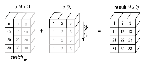
Source: NumPy Documentation

NumPy provides a method broadcast_to, which allows a dense array to be broadcast to a specific shape.

The first task in this phase was to implement a method that replicates this behavior for COO arrays. However, it’s important to note that while NumPy generates a "view" of the original array, the method we introduced instantiated a new coo_array object whose data and coords attributes were generated by tiling and repeating the original array's data and coords. This distinction is important because creating a view, as in NumPy, avoids duplicating data in memory, which is especially relevant when dealing with large arrays. In contrast, creating a new object (as we do here) involves copying the data, which can be more memory- and computation-intensive. For more details on copies and views in NumPy, see this documentation.

matmul

When multiplying matrices A and B, we require that the number of columns of A == number of rows of B, i.e. A has shape (m,n) and B has shape (n,p). But what about multiplying arrays which have more than two dimensions? In this case, we broadcast both arrays over the leading dimensions (those before the last two). The last two dimensions are treated as matrices and must satisfy the matrix multiplication rule, while the remaining dimensions are broadcasted as needed.

If A has shape (..., m, n) and B has shape (..., n, p), the result will have shape (..., m, p) after performing matrix multiplication on the last two dimensions of A and B. If the leading dimensions are not the same, broadcasting applies to make them compatible by expanding dimensions where necessary according to certain rules (see more on broadcasting).

Example:

Let A have shape (4, 5, 1, 3, 6) and B have shape (1, 9, 6, 7). The product's shape will end in (3, 7) (as (m,n) × (n, k) -> (m, k)). We then compare the leading dimensions of A and B, (4, 5, 1) and (1, 9) and expand the dimensions such that both arrays have the same leading dimensions: (4, 5, 9). Now, we can broadcast A from shape (4, 5, 1, 3, 6) to (4, 5, 9, 3, 6), and B from shape (1, 9, 6, 7) to (4, 5, 9, 6, 7).

Developing functionality for matmul involved considering two cases:

1. Multiplication of a sparse array by a sparse array - In this case, we first broadcast both arrays, then convert them to block-diagonal form in COO format (using helper function _block_diag). Afterward, we convert the 2D block-diagonal arrays into CSR format and use csr_matmat for efficient 2D sparse-sparse matrix multiplication, and convert the 2-D block diagonal product to an n-D COO array (using _extract_block_diag) to obtain the final result.

   The process may be better understood through the following code:

   
   

   # Determine the new shape to broadcast A and B

   broadcast_shape = np.broadcast_shapes(shape_A[:-2], shape_B[:-2])

   new_shape_A = broadcast_shape + shape_A[-2:]

   new_shape_B = broadcast_shape + shape_B[-2:]

   A_broadcasted = A.broadcast_to(new_shape_A)

   B_broadcasted = B.broadcast_to(new_shape_B)

   # Convert n-D COO arrays to 2-D block diagonal arrays

   A_block_diag = _block_diag(A_broadcasted)

   B_block_diag = _block_diag(B_broadcasted)

   # Use csr_matmat to perform sparse matrix multiplication

   C_block_diag = (A_block_diag @ B_block_diag).tocoo() # calls 2-D COO matmul, which routes via CSR

   product_shape = broadcast_shape + (A.shape[-2], B.shape[-1])

   # Convert the 2-D block diagonal array back to n-D

   C = _extract_block_diag(C_block_diag, shape=product_shape)

   return C

   
   

2. Multiplication of a sparse array by a dense array - First, we broadcast A and B, then we call a C++ function coo_matmat_dense_nd which performs n-D sparse-dense multiplication (this is the n-D extension of the 2-D function coo_matmat_dense which I added in PR #21240).

   Without diving too deep into the C++ logic, I want to introduce the concept of strides with the following code snippet:

   
   

   std::vector<npy_int64> strides(n_dim);

   strides[n_dim - 1] = 1;

   for (npy_int64 i = n_dim - 2; i >= 0; --i) {

   strides[i] = strides[i + 1] * shape[i + 1];

   }

   
   

   This code creates an array strides, which stores the step size needed to move from one element to the next along a particular axis in a multi-dimensional array. Here, shape is a tuple of dimension sizes of the array.

   There are two common approaches for storing matrices/arrays in memory, namely column-major and row-major ordering. C and C++ use row-major ordering, meaning elements of a row are stored contiguously in memory. This ordering determines how strides are defined for traversing the array.

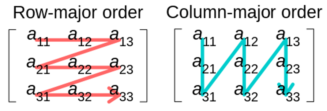
Source: Wikipedia Commons, authored by CMG Lee

dot/tensordot

• Dot

  1. Dot of a sparse array with a sparse array - To compute the dot product of two n-D COO arrays A and B, we map them to 2-D COO arrays using np.ravel_multi_index, convert these arrays to CSR format, and then use csr_matmat. This yields a 2-D result, which is then mapped back to an n-D COO array using np.unravel_index to obtain the final n-D output. This approach was inspired by Dan Schult's proof-of-concept, and was also discussed in #21169 (comment).

  2. Dot of a sparse array with a dense array - This implementation involves reshaping A and B and then using matmul.

     For example: For A of shape (2,3,4,5) and B of shape (6,7,5,9) (where A.shape[-1] == B.shape[-2]), A.dot(B) will have shape (2,3,4,6,7,9). But reshaping A to (2,3,4,1,1,1) and B to (1,1,1,6,7,9) and multiplying the reshaped arrays after broadcasting, we obtain a product of shape (2,3,4,6,7,9), which matches the dot product of the original arrays.

     Routing dot via matmul here had a significant advantage - it avoided the need to introduce new compiled code to handle the sparse-dense case.

• Tensordot

  1. Tensordot of a sparse array with a sparse array - This implementation is similar to that of dot, except that tensordot also takes an axes argument, which requires extra handling. While mapping to 2D for dot, the first dimension consisted of the coordinates obtained from mapping all non-reduced axes to 1D, and the second dimension consisted of the coordinates corresponding to the reduced axis (the rightmost one). In tensordot however, since multiple axes can be reduced, we separately raveled the coordinates for non-reduced and reduced axes to form the 2-D array. The steps for dot then followed.

  2. Tensordot of a sparse array with a dense array - This implementation is also similar to dot's, but involves some additional processing. Unlike dot, where the last dimension is always the reduced one, tensordot can take a tuple of axes to be reduced. Thus, we cannot directly use dot. Instead, we accumulate all reduced axes into one dimension and make this the trailing (rightmost) dimension. The approach taken for this involved transposing the array with a permutation based on the axes argument, so that all the reduced axes became the trailing axes of the transposed array. This was followed by a reshape, where the non-reduced axes remained as they were, but the reduced ones were contracted into a single dimension with a size equal to the product of the dimension sizes of the reduced axes.

     This was definitely one of my favourite ideas that I came up with and worked around - the transposing and permuting involved lots of experimentation with NumPy arrays, until it all fell into place!

This concluded the work for the second PR. Moving on to the third stage, I focused on implementing element-wise operations such as multiply, divide, minimum, maximum, all boolean comparators (==, !=, >, <, >=, <=) etc. The pre-existing behaviour of these was based on a straightforward logic - two arrays could only undergo element-wise operations if they had the same shape. Most of these operations converted the input arrays to CSR/CSC format before further computation. However, at that time, 2-D CSR broadcasting didn't exist, and the need for this to eventually be introduced went all the way back to this issue from 2013. The goal was to ensure that the behaviour of methods in SciPy sparse replicated that of the corresponding NumPy methods.

The work for this PR, therefore, started off by opening a PR to add CSR broadcasting. This followed by making a number of tweaks to the pre-existing CSR/CSC methods, which included removing outdated tests which no longer raised an error, now that 1D and 2D CSR arrays could be multiplied without resulting in a ValueError, provided they were broadcastable. Ensuring that CSR arrays could broadcast before making changes to the COO codebase was essential for maintaining consistency in behaviour across all sparse array formats.

Since COO broadcasting had already been implemented in the second PR, extending most element-wise operations to n-D followed a standard procedure. This involved broadcasting the input arrays, reshaping them to 2-D, routing via CSR, and then reshaping the output back. This update also necessitated modifying the definitions of addition and subtraction to incorporate broadcasting. This led to a change in the definition of densification for COO arrays (performed by the constructor toarray(), one of the first methods defined).

Initially, addition for 1D/2D COO arrays used a C++ function, coo_todense, which was extended to coo_todense_nd for n-D operations. However, since we eventually implemented other element-wise operations by mapping n-D to 2-D and routing via CSR for efficiency, it made sense to apply the same approach to addition. This then removed the usage of coo_todense_nd in addition, and the C++ function was now only called by the toarray() constructor. Replacing any compiled code with Python code is always a plus, as long as the performance isn't affected significantly. This is when I revisited the densification method proposed in Dan Schult's proof-of-concept, which purely utilised NumPy tools. The definition was as follows:

Benchmarking showed that the pure Python code outperformed the compiled version, due to NumPy’s highly optimised array operations (refer to benchmarking results here).

This new toarray() definition was then incorporated, and since coo_todense_nd was no longer needed, it was removed.

After extending the element-wise operations, work was done on adding n-D support for functions like max, min etc., which required carefully mapping to 2-D based on the axes argument using np.ravel_multi_index, followed by routing via CSR. Additionally, I developed constructors such as hstack, vstack, block_diag, and others.

Further enhancements included extending the Kronecker product (kron) and diagonal method to n-D, and introducing tensorsolve in scipy.sparse.linalg, which replicated the behaviour of np.linalg.tensorsolve but for n-D COO arrays. This is an n-D extension of the existing spsolve method in scipy.sparse.linalg, which solves the linear system Ax=b for sparse matrices (2-D) and vectors (1-D).

Testing

Testing was conducted in parallel to the development of each method. This was essential because minor changes in one file can potentially break functionality across the entire SciPy codebase. To address this, it was important to ensure that all functionalities remained intact across the module and that no tests failed due to recent changes or added code.

For methods such as add, sub, max, nanmax etc., it was vital to ensure that correct behaviour was observed when given input data such as empty arrays, shapes with dimension size of 0, data with NaN and inf values, and empty tuple () arguments. Operations like matmul and tensordot required boundary condition testing and validation across all possible dimension combinations (e.g., 1D * 3D, 6D * 1D, 4D * 2D).

---

Status

At the time of writing, the first PR has been merged, the second PR is under review by the maintainers, and the final segment of work is complete. This segment will be submitted once the previous PR is merged. The scheme of action for this work will depend on whether the community prefers breaking down different sections of the work into individual PRs to facilitate the review process.

The tracker issue will be updated with progress as further PRs are merged.

Acknowledgements

This internship has been an incredible learning experience, and this wouldn't have been possible without the exceptional guidance and support that I received from my mentors, Ralf Gommers and Irwin Zaid. I also want to express my gratitude to the SciPy community, particularly Dan Schult and CJ Carey for their involvement in reviewing many of my PRs, and to Melissa Weber Mendonça for coordinating this program and providing support throughout the internship. I am very grateful for this opportunity. Knowing that my contributions will be part of a widely used package like SciPy is a significant motivation!

References

• Proof-of-concept for n-D sparse arrays
• Tracker Issue for n-D COO array support in SciPy
• The array API standard