Unlocking C-level performance in pandas.DataFrame.apply with Numba

Introduction

If you've been using pandas for a while, you are probably familiar with the family of apply functions in pandas (e.g. DataFrame.apply, Series.apply, DataFrameGroupBy.apply, etc.). For those unaware, these functions allow you to specify a Python function to be called for each row/column of a DataFrame, and then combines and returns the results back to you.

Because everything happens in Python-land, though, apply is usually very slow. It's recommended that you only use it when you cannot find an equivalent method that does what you want.

In pandas 2.2.0 however, a new engine (engine="numba") option will be added to DataFrame.apply, opening up the possibility for fast and parallelizable apply in pandas. It works by using Numba, a JIT (just-in-time) compiler that translates your Python/NumPy functions into fast machine code when their called, providing up to a compared to the original python engine.

So, can I just slap on engine="numba" to DataFrame.apply and enjoy a free many-times speedup?


- df.apply(f)
+ df.apply(f, engine="numba")

Well, not quite. Because of the way that Numba and the numba engine inside pandas work, there are several caveats to keep in mind to obtain this speedup.

TL;DR: Use apply only when you have to (e.g. there is no corresponding method or chain of pandas methods that do that you want). If you absolutely have to, then engine='numba' may help get better performance

How the Numba engine works

Currently, in pandas, there are currently two implementations of the Numba engine inside of apply, one for raw=True, and one for raw=False (the default).

If you didn't know already, passing in raw=True to DataFrame.apply tells pandas to pass in NumPy arrays, not pandas Series, to the functions you pass into apply. Because Numba itself supports NumPy arrays natively, in general, every function runnable with the python engine should also be runnable with the numba engine, as long as you stick to the supported NumPy features inside Numba.

When raw=False, apply operates on the pandas Series representations of rows/columns, which won't work by default, since Numba doesn't recognize pandas objects or functions. We could work around this by breaking down DataFrame/Series into their values and indices (like we do in Groupby methods that support Numba user-defined functions (UDFs), e.g. transform). Unfortunately, this approach would require users to rewrite their code to use Numba, which can be a pretty big barrier to adoption.

To work around this limitation, we can use Numba's extension API, to teach Numba to operate on pandas Series/DataFrames. In essence, what we can do through this API, is define a equivalent data structure for the internals of a pandas Series inside Numba, and also define Numba equivalents of the pandas Series methods that we want. Through this, we can create a "mocked" version of a pandas Series, that JITed Numba code can access. Now, we can create pandas Series inside Numba. Finally, we need to define a way to convert to and from the Numba representation by using Numba's boxing/unboxing APIs, which is fairly straightforward as we can unwrap NumPy-backed Series into NumPy arrays, for the index and for the values.

One thing that's important to note with this approach is that these APIs usually operate at a pretty low level and, as per usual for Numba code, we have no access to the original pandas Python object in Numba-land. This means that whatever we don't define in our mocked dataframe will not be available to use in a JITed Numba function and will raise an error at compile-time (see the "supported features" section below for more info).

If you're curious about what this looks like, check out the implementation in pandas to learn more.

Supported features

To summarize the existing support as of pandas 2.2.0, the numba engine in df.apply supports:

Numeric columns/rows
Series methods *
- In general, all methods that have a NumPy equivalent (e.g. mean) are supported
- Other more complex methods are generally unsupported.
Indexing *
- Indexing with a scalar is supported with the Numba engine, but indexing with a slice object or via fancy indexing is not supported.
Basic binary operations
- e.g. addition, subtraction, multiplication, and division
Parallel apply
- This is only supported when raw=True
- Like other functions that support Numba, you can pass in parallel: True inside the engine_kwargs dictionary argument to use apply in parallel.

*: This indicates partial support

Because the Numba engine is still very new and experimental, we don't support DataFrames containing Apache Arrow backed arrays, datetime/timedelta arrays, or string arrays. However, it is anticipated that these and other features will be added, as the Numba engine matures and picks up adoption.

Because of limitations within Numba, the Numba engine will never support:

Any Python/NumPy operations not supported by Numba
- It's important to note that Numba only compiles a subset of valid Python code. Check out the list of supported Python features for more info.
Object dtype arrays
Generic Extension Arrays
Mutation of the original pandas object pandas inside of your function
- This is already discouraged inside of apply, but will not work at all with the Numba engine, and may crash your program.

For these unsupported features, it is recommended that you use the python engine or find an alternative to apply.

Performance

To understand the performance of the new Numba engine, it's helpful to understand the steps going on under the hood when you call apply, and the overhead that each step contributes to the runtime.

Understanding the JIT process

The runtime of apply under Numba consists of 4 parts

JIT compilation with Numba
- This stage will JIT the function that you pass in if it has not been JIT compiled yet, and cache it for future calls.
Unboxing the DataFrame
- During this stage, the DataFrame is converted to a format recognizable to Numba This mostly involves extracting the NumPy arrays backing the DataFrame, and then converting to the Numba representation of a DataFrame. When raw=True, conversion to the Numba representation isn't necessary, as we operate on the NumPy arrays instead.
Running the function
Boxing the DataFrame
- This is the opposite of the unboxing phase, and during this phase, we pack the results of applying the function back into pandas objects.

Note that parts (1), (2), and (4) contribute to the overhead in running the function. Depending on the function you pass into apply, this overhead can be pretty significant. We can see the impact of each one of these overheads in our benchmarks below.

Performance Case Study

Here, we will look at the performance of the Numba engine. The DataFrame we will operate on will be long and narrow (10,000 rows and 3 columns), and we will have a mix of randomly generated integers and floats.

We will perform 4 tests here on:

Analyzing overhead of the Numba engine
Indexing performance of the Numba engine
Analyzing performance of the Numba engine on normalizing rows of a DataFrame
Comparing raw=True and raw=False, and analyzing the speedups provided by parallel execution with the Numba engine when operating on the raw values of the DataFrame.

All tests are performed with Numba 0.58.1.

First let's create our DataFrame.


import pandas as pd
import numpy as np
np.random.seed(42)
size = int(10**4)
df = pd.DataFrame({"a": np.random.randn(size),
                   "b": np.random.randint(0, size, size),
                   "c": np.random.randn(size)})
df.head(3)

	a	b	c
0	0.496714	1897	1.214547
1	-0.138264	5751	0.855936
2	0.647689	5150	-0.533877

3 rows × 3 columns

Measuring compilation and boxing/unboxing overhead

First, to give an idea of how much overhead compilation and boing/unboxing creates, we will use a simple function that returns the input Series without modification.


>>> f = lambda x: x


>>> # Timing the compilation time
>>> # To estimate this, we will use the Numba engine on a very small DataFrames
>>> small_df = pd.DataFrame({"a": [1]})
>>> %time small_df.apply(f, engine="numba", axis=1)
>>> %time small_df.apply(f, engine="numba", axis=1)
CPU times: user 1.97 s, sys: 175 ms, total: 2.15 s
Wall time: 2.43 s
CPU times: user 1.11 ms, sys: 39 µs, total: 1.15 ms
Wall time: 1.14 ms

Notice how the compilation overhead disappears on the second run because of the caching of the compiled function.

Now, let's measure the overhead of the boxing/unboxing of the input DataFrame. To do this, we will compare the speed of apply with Numba with raw=True and raw=False.

Although doing a raw apply on the DataFrame still does have some overhead (mainly due to converting the DataFrame into a 2D ndarray), it is minimal compared to the total execution time.


>>> df.apply(f, engine="numba", axis=1)  # warmup run to avoid JIT compilation
>>> %timeit -n 20 df.apply(f, engine="numba", axis=1)
167 ms ± 901 µs per loop (mean ± std. dev. of 7 runs, 20 loops each)


>>> %timeit df.apply(f, engine="numba", axis=1, raw=True)
236 µs ± 3.77 µs per loop (mean ± std. dev. of 7 runs, 20 loops each)

We can see here that several order of magnitude of difference between raw=True and raw=False. This is because the unboxing process currently individually unboxes each resultant Series to a Python object before concatenating them together to build the result DataFrame.

In future pandas releases, this can be optimized by concatenating the results of apply inside of the Numba engine (which would only require one final unboxing call for the concatenated DataFrame), which should bring the speed of apply on Series in Numba on par with the speed on the raw NumPy arrays.

Despite this, the Numba engine is still able to match the speed of the Python engine:


>>> %timeit -n 20 df.apply(f, engine="python", axis=1)
166 ms ± 1.52 ms per loop (mean ± std. dev. of 7 runs, 20 loops each)

Indexing Performance

Here, we will do a very simple test of selecting a column/row, followed by a more complex example of taking the square of the difference of two columns.


>>> f = lambda x: x['b']
>>> df.apply(f, engine="numba", axis=1)  # warmup run to avoid JIT compilation
>>> %timeit -n 20 df.apply(f, engine="numba", axis=1)
>>> %timeit -n 20 df.apply(f, engine="python", axis=1)
20.1 ms ± 431 µs per loop (mean ± std. dev. of 7 runs, 20 loops each)
38.7 ms ± 302 µs per loop (mean ± std. dev. of 7 runs, 20 loops each)


>>> f = lambda x: x[10]
>>> df.apply(f, engine="numba", axis=0)  # warmup run to avoid JIT compilation
>>> %timeit -n 20 df.apply(f, engine="numba", axis=0)
>>> %timeit -n 20 df.apply(f, engine="python", axis=0)
941 µs ± 14.9 µs per loop (mean ± std. dev. of 7 runs, 20 loops each)
199 µs ± 8.26 µs per loop (mean ± std. dev. of 7 runs, 20 loops each)


>>> # Something a little more advanced
>>> f = lambda x: (x['a'] - x['c']) ** 2
>>> %timeit -n 20 df.apply(f, engine="numba", axis=1)
>>> %timeit -n 20 df.apply(f, engine="python", axis=1)
25 ms ± 6.84 ms per loop (mean ± std. dev. of 7 runs, 20 loops each)
57.1 ms ± 432 µs per loop (mean ± std. dev. of 7 runs, 20 loops each)

Numba outperforms the Python engine when selecting columns by 2-3x, but is slower when selecting rows. This is probably because there are only 3 columns to apply our function to, but in the future this could be optimized to at least be somewhat on par with the Python engine.

Normalization example

Now, let's try a more complicated example where we normalize each row. Here, Numba really shines, providing roughly a 10x speedup over the Python engine.

Note that because Numba only supports ddof=0, we are not using the std method on a Series (since that defaults to ddof=1).


>>> f = lambda x: (x - x.mean()) / np.std(x.values)
>>> # Note: The Python engine takes a bit longer to run the apply, so we're
>>> # reducing the number of runs here.
>>> df.apply(f, engine="numba", axis=1)  # warmup run to avoid JIT compilation
>>> %timeit -n 10 df.apply(f, engine="numba", axis=1)
>>> %timeit -n 10 df.apply(f, engine="python", axis=1)
169 ms ± 1.54 ms per loop (mean ± std. dev. of 7 runs, 10 loops each)
2.18 s ± 114 ms per loop (mean ± std. dev. of 7 runs, 10 loops each)

Your mileage will vary depending on the number of items you're applying on though. Running the same function over the columns, yields only a ~37% speedup, because there are only three columns.


f = lambda x: (x - x.mean()) / (np.std(x.values))
df.apply(f, engine="numba", axis=0) # warmup run to avoid JIT compilation
%timeit -n 20 df.apply(f, engine="numba", axis=0)
%timeit -n 20 df.apply(f, engine="python", axis=0)
708 µs ± 26.6 µs per loop (mean ± std. dev. of 7 runs, 20 loops each)
1.13 ms ± 86.5 µs per loop (mean ± std. dev. of 7 runs, 20 loops each)

Performance comparison between raw=True / raw=False

We will now look at how performance differs with the Numba engine when raw=True and raw=False, using the same normalization function from before. We'll also look at when parallel apply (only available when raw=True) can provide a speedup, compared to regular DataFrame functions.

Previously, we had around 169ms in execution time for raw=False. Now, let's check out the performance with raw=True:


>>> df.apply(raw_f, engine="numba", axis=1, raw=True, engine_kwargs={"parallel": False})  # warmup
>>> %timeit -n 20 df.apply(raw_f, engine="numba", axis=1, raw=True, engine_kwargs={"parallel": False})
1.48 ms ± 70.3 µs per loop (mean ± std. dev. of 7 runs, 20 loops each)

Notice as with before how operating on raw values is much faster than operating on the Series itself. Now, let's trying operating in parallel.

Here, we can see roughly a 6x speedup over just using raw (again, this was performed on my 2019 Intel MacBook Pro with 6 cores):


>>> df.apply(raw_f, engine="numba", axis=1, raw=True, engine_kwargs={"parallel": True})  # warmup
>>> %timeit -n 20 df.apply(raw_f, engine="numba", axis=1, raw=True, engine_kwargs={"parallel": True})
OMP: Info #276: omp_set_nested routine deprecated, please use omp_set_max_active_levels instead.
289 µs ± 15.5 µs per loop (mean ± std. dev. of 7 runs, 20 loops each)

Finally, for comparison's sake, let's look at the Python performance with raw=True, and also the time it takes for the vectorized equivalents:


>>> %timeit -n 20 df.sub(df.mean(axis=1), axis=0).div(df.std(ddof=0, axis=1), axis=0)
3.25 ms ± 600 µs per loop (mean ± std. dev. of 7 runs, 20 loops each)

In this case, parallel apply with raw=True provided a good speedup (~10x), however, this is not guaranteed to happen in all cases.

A good rule of thumb to follow is that if there already exists a NumPy/pandas function that does what you want to do already, you should use that, as it is hard for Numba to beat the optimized low-level routines in both of those libraries.

However, if your operation chains together a lot of these operations, Numba may still provide a pretty good speedup. For example, in our normalization example above, we took the mean, did a subtraction, took the standard deviation, and then did a division. Because NumPy evaluates each one of these operations eagerly, it may miss out on performance optimizations that the Numba compiler is able to use, explaining the performance improvement with Numba above.


>>> # Let's take a look at the performance of just a mean operation with Numba
>>> # (both raw mode and parallel on)
>>> # and just with numpy/pandas
>>> f = lambda x: x.mean()
>>> df.apply(f, engine='numba', raw=True, engine_kwargs={'parallel': True}, axis=1)  # warmup
>>> %timeit -n 20 df.apply(f, engine='numba', raw=True, engine_kwargs={'parallel': True}, axis=1)
>>> %timeit -n 20 df.mean(axis=1)
>>> %timeit -n 20 df.values.mean(axis=1)
160 µs ± 24.4 µs per loop (mean ± std. dev. of 7 runs, 20 loops each)
1.59 ms ± 60 µs per loop (mean ± std. dev. of 7 runs, 20 loops each)
77.8 µs ± 6.11 µs per loop (mean ± std. dev. of 7 runs, 20 loops each)

Here, we can see that although Numba beats the pandas mean function by ~10x, it's 2x slower than the NumPy version, illustrating the point above.

To conclude our analysis, let's finish with a log-log plot running the normalization example for various DataFrame sizes (here, we do up to 1,000,000 rows, but you can run the script for larger sizes yourself if you'd like):


import matplotlib.pyplot as plt
f = lambda x: (x - x.mean()) / (np.std(x.values))
raw_f = lambda x: (x-x.mean()) / x.std()
def time_numba(timing_func, func_name, save=False):
    def time_sizes(kwargs, engine_kwargs, n_loops=200):
        times = []
        for size in sizes:
            times.append(timing_func(size, kwargs=kwargs, engine_kwargs=engine_kwargs, n_loops=n_loops))
        return times
    # Running for sizes about: 500, 1k, 15k, 130k, ~1mil
    sizes = [2**7, 2**9, 2**10, 2**14, 2**17, 2**20]
    fig, ax = plt.subplots(nrows=1, ncols=1, figsize=(8, 6))
    full_kwargs = [({"engine": "python"},{}),
                     ({"engine": "numba", "raw": False},{}),
                     ({"engine": "numba", "raw": True},{}),
                     ({"engine": "numba", "raw": True},{"parallel": True})]
    # We also set `n_loops`, otherwise # the Python engine will take way too
    # long on the larger sizes.
    n_loops_lst = [1, 1, 1, 1]
    for (kwargs, engine_kwargs), n_loops in zip(full_kwargs, n_loops_lst):
        label_dict = kwargs.copy()
        label_dict.update(engine_kwargs)
        ax.loglog(sizes, time_sizes(kwargs, engine_kwargs, n_loops), 'o-', label=str(label_dict))
        ax.grid(True)
        ax.set_xlabel('DataFrame size')
        ax.set_ylabel('Time taken')
        ax.set_title('{}'.format(func_name))
    ax.legend(loc='best', numpoints=1)
    if save:
        fig.savefig('benchmark_numba_{}.png'.format(func_name))
    return fig, ax
def time_normalization(size, kwargs, engine_kwargs, n_loops):
    df = pd.DataFrame({"a": np.random.randn(size),
                       "b": np.random.randint(0, size, size),
                       "c": np.random.randn(size)})
    if "raw" in kwargs and kwargs["raw"]:
        func = raw_f
    else:
        func = f
    namespace = locals().copy()
    expr = "df.apply(func, axis=1, **kwargs, engine_kwargs=engine_kwargs)"
    return min(timeit.repeat(expr, number=n_loops, globals=namespace)) / n_loops
fig, axes = time_numba(time_normalization, 'Scaling of apply with normalization UDF', save=False)
plt.show()

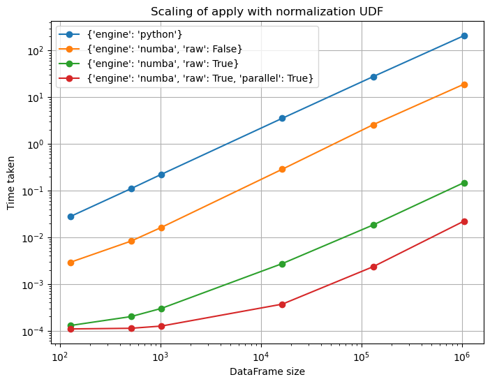
A log log plot of the normalization function being ran with various sizes

As we can see, the Numba engine is pretty consistently faster than the Python engine from the get go, even from small sizes of ~100 rows. Parallel mode also matches the speed of the non-parallel mode at small sizes (for this particular function at least, you might see a slowdown for others), and starts to provide good speedups for DataFrames with greater than 10,000 rows.

Conclusion

All in all, the Numba engine will offer a faster way for pandas users to run their apply functions with minimal changes, for functions containing standard pandas operations (think indexing, arithmetic, and using NumPy functions on the data) in pandas 2.2 and above.

It does this by "mocking" the Series object passed in to your function. This is necessary because Numba code cannot access the methods on a Series like Python code can - each Numba equivalent must either be rewritten or wrap the logic behind the original method. For users, this means that some Series functionality may be missing from the "mocked" Series object, so not all functions will compile out of the box with the "numba" engine.

The numba engine also opens up the door to parallel DataFrame.apply when operating on the raw values of the DataFrame (with raw=True), which is super exciting as this has been a highly requested feature in pandas over the years. It's important to note that this may not always result in a performance speedup over using the "vectorized" pandas/numpy equivalents of your function (it it exists), and it's always recommended to at least attempt to vectorize your function before trying out the numba apply engine, and its various modes(e.g. raw, parallel, etc.).

While many features/methods may be missing from the mocked Series object currently (such is the nature of mocking) and the Numba engine in general, it's expected that these will slowly be added in as the Numba engine is adopted, and from contributions from users like you!

Acknowledgements

I'd like to thank Matthew Roeschke for reviewing my PRs, and the Numba developers for helping to answer my questions about Numba. I'd also like to thank Ralf Gommers and Marco Gorelli for peer reviewing this blog post.

This work was supported by a grant from NASA to Pandas, scikit-learn, SciPy and NumPy under the NASA ROSES 2020 program.